Scaling, Reliability, and Cost

Planning Capacity and Preserving Service Quality Under Changing Load

Scaling, Reliability, and Cost

Chapter 06 established how to detect and coordinate a response when production behaviour threatens the service-level objective (SLO). A dependable system should also reduce the probability that ordinary demand becomes an incident. That requires enough capacity, controlled elasticity, bounded work, and failure isolation.

Scaling is not the same as adding replicas. A system scales successfully when it sustains its user-facing promise as workload changes. A configuration that processes more requests but violates latency, creates an unbounded queue, or multiplies cost without improving useful throughput has not solved the operational problem.

This chapter continues the decision API case study. The service receives uneven traffic, each replica has a measured performance limit, new replicas require time to become ready, and at least one replica must be allowed to fail without exhausting capacity. The practical exercise compares fixed capacity, reactive autoscaling, and demand-aware autoscaling using the same workload.

Learning objectives

By the end of this chapter, you should be able to:

• translate a workload forecast and load-test result into a replica requirement;
• distinguish horizontal, vertical, workload, and node scaling;
• select scaling signals that represent demand rather than symptoms;
• explain how queues, timeouts, retries, load shedding, and circuit breakers interact;
• preserve reliability during failures and planned disruptions;
• compare performance, reliability, and cost with unit-level measures; and
• define a capacity and autoscaling policy for the case-study API.

Capacity begins with demand

Capacity planning connects an expected workload to the resources required to meet a service objective. It is not a one-time estimate. Demand, code, models, dependencies, instance types, and performance targets all change.

Begin by describing the work rather than the infrastructure:

• requests per second and requests per hour;
• concurrent requests;
• payload size and response size;
• input-validation, preprocessing, inference, and policy costs;
• batch size, when batching is safe;
• daily and weekly patterns;
• burst size and duration;
• regional or tenant concentration; and
• expected growth and exceptional events.

Average traffic is insufficient. A service averaging 30 requests per second may reach 130 requests per second during a five-minute burst. Provisioning for the average creates a predictable incident.

Measure one replica under realistic conditions

Load testing should establish a performance envelope for one representative replica. Increase concurrency gradually and record:

• completed throughput;
• p50, p95, and p99 latency;
• error and timeout rates;
• CPU, memory, accelerator, and connection use;
• queue depth and wait time; and
• downstream dependency behaviour.

The useful limit is not the highest throughput observed before the process crashes. It is the highest sustained throughput that still meets the latency and error objectives. In the exercise, one replica can physically complete about 32 requests per second, but operating near that boundary causes sharp latency growth. The planning target is therefore 65% utilization:

\[ C_{\text{planned}} = C_{\text{measured}} \times U_{\text{target}} = 32 \times 0.65 = 20.8 \text{ requests/second}. \]

If forecast peak demand is \(D\), the basic replica estimate is

\[ N_{\text{load}} = \left\lceil \frac{D}{C_{\text{planned}}} \right\rceil. \]

For 130 requests per second, \(N_{\text{load}} = \lceil 130 / 20.8 \rceil = 7\). If the service must tolerate one unavailable replica, provision eight:

\[ N_{\text{required}} = N_{\text{load}} + N_{\text{failure reserve}} = 8. \]

This arithmetic is a starting point. Shared dependencies may become the actual bottleneck before eight replicas are useful. Validate the complete system at the expected aggregate load.

Concurrency and service time

Throughput alone can hide why a service saturates. Little’s Law relates average concurrency \(L\), arrival rate \(\lambda\), and average time in the system \(W\):

\[ L = \lambda W. \]

At 100 requests per second and 0.2 seconds per request, average in-flight work is 20 requests. If service time rises to 0.8 seconds while arrivals remain constant, concurrency rises to 80. More work then competes for the same connections, memory, and workers. This feedback is one route from a slow dependency to cascading failure.

Use percentiles as well as averages. An acceptable mean can coexist with a harmful tail, especially when one user workflow makes several dependent calls.

Horizontal and vertical scaling

There are two primary workload-level scaling directions.

Horizontal scaling

Horizontal scaling changes the number of service replicas. It works well when instances are interchangeable and request state is stored externally or can be reconstructed.

Advantages include failure isolation, gradual changes, rolling replacement, and a large scaling range. Costs include load-balancing complexity, duplicated model memory, cold starts, and pressure on shared dependencies.

Model artifacts can make horizontal scaling expensive. If each process loads a 3 GB model, eight replicas may require 24 GB before accounting for runtime memory. Shared model servers, process-level copy-on-write, batching, quantization, or a smaller approved model may improve economics, but each option changes performance or operational risk and must be measured.

Vertical scaling

Vertical scaling changes CPU, memory, or accelerator resources assigned to an instance. It can be appropriate when the workload cannot be partitioned efficiently, the model needs a larger memory footprint, or per-replica overhead dominates.

Vertical capacity has a ceiling and can concentrate failure impact. Resource changes may also require replacement or rescheduling, depending on the platform and feature set. Kubernetes supports both horizontal workload autoscaling and vertical autoscaling; the latter may update requests or replace workloads according to its mode (The Kubernetes Authors 2026a, 2026e).

Combine the two deliberately

A common pattern is to right-size replicas vertically, then scale their count horizontally. Right-sizing provides a stable unit of capacity. Horizontal scaling handles demand variation and instance failure.

Avoid letting independent vertical and horizontal controllers react aggressively to the same signal. One controller may increase replica size while another increases replica count, creating oscillation and unpredictable cost. Establish ownership, compatible time scales, and limits.

Requests, limits, and scheduling

Resource configuration affects both performance and whether replicas can be scheduled.

• A request represents the resource quantity used for placement and reservation decisions.
• A limit bounds resource use according to the platform’s enforcement mechanism.
• Observed use is what the process actually consumes under a particular workload.

Requests that are too low can pack too many replicas onto a node and create contention. Requests that are too high can leave expensive capacity unused and prevent new replicas from scheduling. A tight CPU limit may throttle work and increase latency; an inadequate memory limit can cause termination under peak use.

Set initial values from load-test evidence, observe throttling and memory high-water marks, and revise them after material application or model changes. Node capacity must also be able to satisfy new replicas. Workload autoscaling without corresponding node capacity can produce pending replicas rather than useful capacity; Kubernetes documents combining horizontal workload autoscaling with node autoscaling for this reason (The Kubernetes Authors 2026c).

Autoscaling is a feedback controller

An autoscaler observes a signal, calculates desired capacity, and changes the system. Every part of that loop has delay:

demand changes -> metric is emitted -> metric is collected -> controller decides
               -> replica is scheduled -> model loads -> readiness succeeds

If the complete delay is four minutes, reactive scaling cannot protect the first four minutes of a sudden burst. Minimum capacity, scheduled scaling, fast startup, a bounded queue, or admission control must absorb that interval.

Kubernetes Horizontal Pod Autoscaling uses a ratio between current and desired metric values to calculate desired replicas, conceptually (The Kubernetes Authors 2026b):

\[ N_{\text{desired}} = \left\lceil N_{\text{current}} \times \frac{M_{\text{current}}}{M_{\text{target}}} \right\rceil. \]

Choose a signal close to demand

CPU is useful when CPU use increases consistently with request load and does so before the SLO fails. It is weak when inference is memory-bound, waits on a remote feature service, or uses an accelerator invisible to the CPU signal.

Possible scaling signals include:

Signal	Strong use	Main caution
CPU utilization	CPU-bound, homogeneous requests	May lag or ignore dependency waits
In-flight requests	Concurrency-limited APIs	Requires a validated per-replica target
Queue depth or oldest age	Asynchronous workers	A growing queue may already indicate harm
Requests per second	Similar request cost	Expensive and cheap requests are treated equally
Accelerator utilization	GPU-bound inference	Batching can make the relationship nonlinear
Scheduled demand	Predictable peaks	Forecast error requires reactive protection

Latency and error rate are usually late signals: scale before they violate the SLO. Keep them as safety gates even when another measure controls replicas.

Define controller behaviour

An autoscaling policy should specify:

• minimum and maximum replicas;
• target metric and aggregation window;
• scale-up step or rate;
• scale-down stabilization window;
• startup and readiness time;
• missing or delayed metric behaviour;
• a manual override; and
• what happens when maximum capacity is reached.

Scale up quickly enough to contain harm, but scale down conservatively. Rapid scale-down can remove the headroom needed for a recurring burst and cause thrashing. Never scale to zero on a latency-sensitive synchronous pathway unless the cold-start delay is explicitly acceptable.

Illustrative configuration

The following manifest shows the intent, not a universal production default:

apiVersion: autoscaling/v2
kind: HorizontalPodAutoscaler
metadata:
  name: decision-api
spec:
  scaleTargetRef:
    apiVersion: apps/v1
    kind: Deployment
    name: decision-api
  minReplicas: 2
  maxReplicas: 8
  behavior:
    scaleUp:
      stabilizationWindowSeconds: 0
      policies:
        - type: Percent
          value: 100
          periodSeconds: 60
    scaleDown:
      stabilizationWindowSeconds: 600
      policies:
        - type: Percent
          value: 25
          periodSeconds: 60
  metrics:
    - type: Resource
      resource:
        name: cpu
        target:
          type: Utilization
          averageUtilization: 65

The maximum of eight reflects the exercise’s tested capacity and failure reserve. A maximum must not be chosen only from budget: it should also respect cluster capacity, dependency quotas, and the highest scale validated by load testing.

Reliability under pressure

Elasticity cannot be the only overload defence. It may be slow, unavailable, or limited by a dependency. Reliable systems bound the amount of work admitted and the time spent on it.

Bound queues

An unbounded queue converts overload into rising latency and memory use. When arrival rate remains above completion rate, the queue cannot recover without reducing arrivals or increasing effective service capacity.

Set a maximum queue length or wait time. When the bound is reached, reject new work clearly, shed low-priority work, or route it to a safe alternative. For asynchronous work, monitor the age of the oldest item as well as queue length.

Use deadlines and timeouts

Every remote call should have a timeout derived from the end-to-end deadline. A client with a 500 ms deadline cannot safely allow one dependency to wait for 2 seconds. Timeouts release resources, but they do not necessarily cancel work already executing downstream; cancellation propagation should be tested.

Retry selectively

Retries can recover from brief transient failures, but they also multiply load. Three layers each attempting three retries can turn one user request into many downstream attempts. Retry only operations that are safe to repeat, use exponential backoff with jitter, cap the attempt count, and keep retry time within the original deadline.

Google’s SRE guidance warns that positive feedback—overload causing errors, retries causing more load, and slower responses retaining resources longer—can produce cascading failure (Beyer et al. 2026). Place retry responsibility at one appropriate layer and use a retry budget.

Isolate failures

Use separate worker pools, connection pools, queues, or concurrency limits when one workload class could consume all resources. This bulkhead pattern preserves capacity for critical traffic.

A circuit breaker stops sending work to a dependency that is repeatedly failing, then allows limited probes during recovery. It should expose its state in telemetry and define a safe fallback. A circuit breaker that silently returns stale or fabricated predictions trades availability for correctness without acknowledging the decision risk.

Shed load intentionally

When capacity is exhausted, partial service can be safer than universal collapse. Possible policies include:

• reject non-critical batch requests before synchronous decisions;
• enforce per-client quotas;
• move ambiguous cases to manual review;
• serve a validated lower-cost model where policy permits;
• return a clear retryable response; or
• fail closed for safety-critical decisions.

The policy is a product and governance decision, not merely an infrastructure setting.

Reliability during instance and node loss

Replica count alone does not establish redundancy. Eight replicas placed on one node share one failure domain. Spread replicas across nodes and, where required, zones. Use topology constraints or anti-affinity, but verify that the cluster has enough distinct capacity to satisfy them.

Readiness should remove an unhealthy instance from traffic before users encounter repeated failures. Graceful shutdown should stop new requests, allow bounded in-flight work to finish, and then terminate. Termination grace periods must be consistent with the load balancer’s draining behaviour and request deadlines.

Planned maintenance also consumes redundancy. A PodDisruptionBudget can limit concurrent voluntary disruption for a replicated Kubernetes application, but it does not create capacity and does not protect against every involuntary failure (The Kubernetes Authors 2026d). Keep enough ready replicas to satisfy both the user load and the allowed disruption.

Test failure assumptions deliberately:

• terminate one replica during peak load;
• drain a node;
• delay or fail a dependency;
• prevent new nodes from provisioning;
• corrupt or withhold an autoscaling metric; and
• reach the configured maximum replica count.

The result should be evidence about user impact, detection time, controller response, and recovery—not merely confirmation that the platform replaced a process.

Performance and cost are joint constraints

The cheapest configuration that violates the SLO is not efficient. The most reliable configuration at any price may be financially unsustainable. The objective is to deliver the required service quality at a defensible unit cost.

Track cost in dimensions that connect infrastructure to useful work:

\[ \text{cost per 1,000 successful decisions} = \frac{\text{allocated service cost}} {\text{successful decisions}} \times 1000. \]

Useful companion measures include:

• cost per request and per completed workflow;
• cost per manually reviewed case;
• accelerator-seconds per prediction;
• idle cost required for failure reserve;
• cost of retries and rejected work; and
• cost by model version, endpoint, tenant, or environment.

The FinOps Foundation recommends connecting technology spend to meaningful units such as transactions or model runs so changes can be interpreted as efficiency gains or runaway cost drivers (FinOps Foundation 2026). Unit cost must be paired with SLO attainment: a falling unit cost caused by timeouts or lower-quality decisions is a false improvement.

Practical optimization order

1. Remove unused resources and abandoned environments.
2. Measure and right-size requests, limits, replicas, and storage.
3. Improve code, queries, serialization, batching, or model execution.
4. Use elasticity for variable demand while preserving minimum headroom.
5. Select a more suitable instance or accelerator.
6. Consider commitments only for a stable baseline after usage is understood.

Discounts can reduce the price of waste without improving efficiency. Optimize the architecture and usage before treating purchasing terms as the primary solution.

Practical exercise: compare capacity policies

The supporting program creates a deterministic three-hour workload with a short surge and a larger scheduled peak. It compares:

• fixed capacity: four replicas throughout;
• reactive autoscaling: two to eight replicas, responding after a four-minute readiness delay; and
• demand-aware autoscaling: the same bounds, but scheduled demand provides nine minutes of lead time while reactive control remains active.

Run it from the repository root:

bash scripts/bash/07-simulate-scaling-and-cost.sh

or directly:

python scripts/python/07-simulate-scaling-and-cost.py

The program writes:

results/07-scaling-simulation.csv
results/07-scaling-summary.csv
results/figures/07-capacity-and-cost.png
results/figures/07-reliability-under-load.png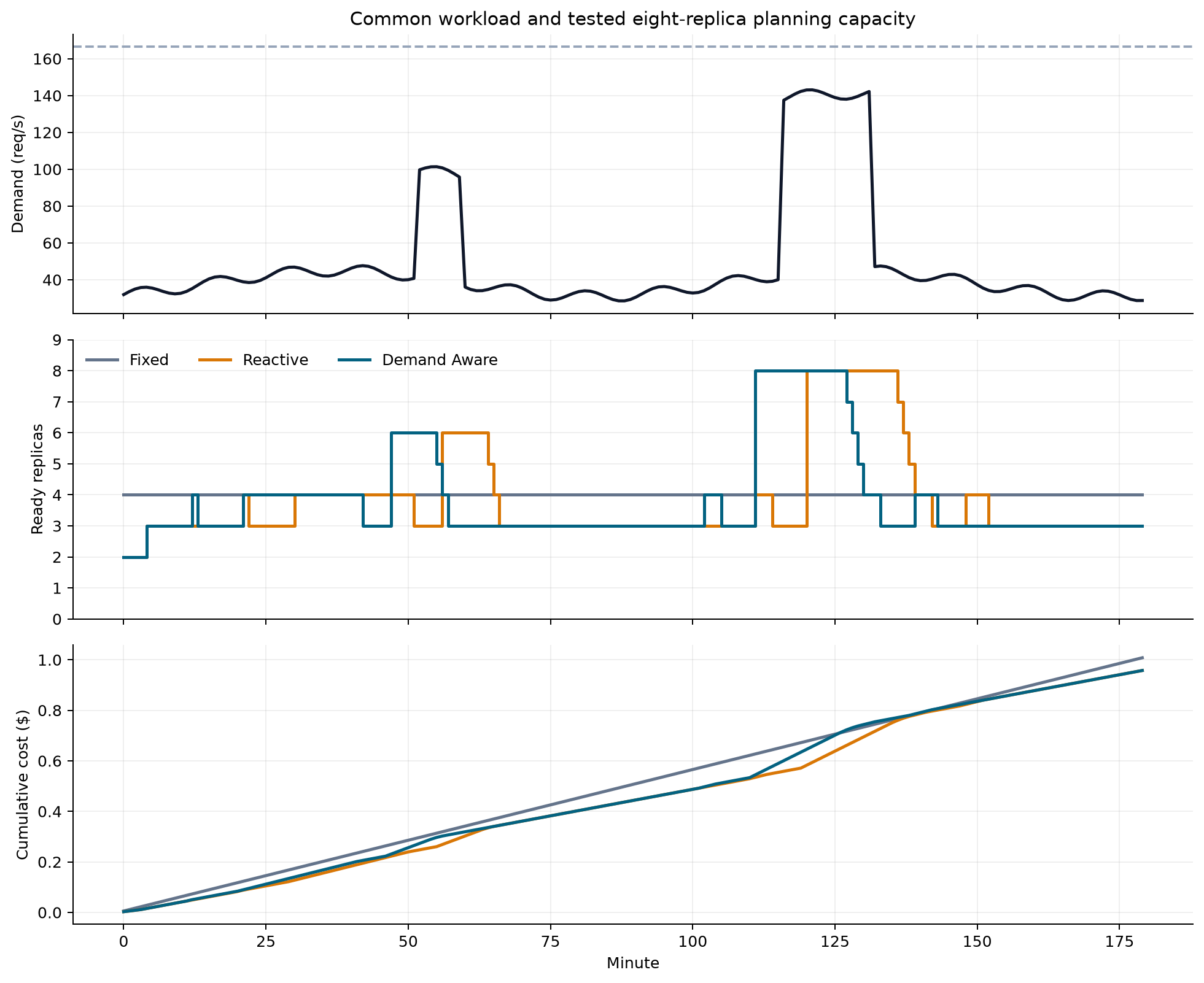

Figure 9.1: Demand, ready replicas, and cumulative compute cost for three capacity policies.

Figure 9.1 makes the control delay visible. Reactive scaling eventually reaches sufficient capacity but cannot create ready replicas before it observes the demand. Demand-aware scaling uses the known peak schedule to act earlier. Its forecast is not trusted alone: minimum capacity and reactive correction remain in place.

Figure 9.2: Utilization, p95 latency, and cumulative rejected requests under the same scaling policies.

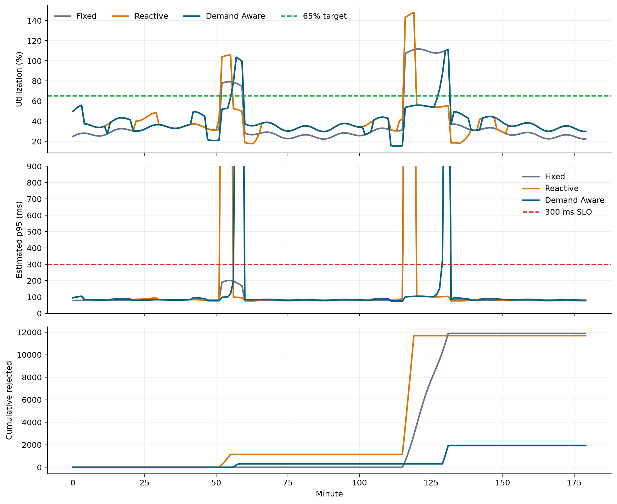
The simulation deliberately separates planned capacity from physical capacity. A replica can process up to 32 requests per second, but the scaling target reserves headroom by planning around 20.8. Latency increases before physical exhaustion, and requests above physical capacity are rejected rather than placed in an unbounded queue.

Inspect the summary:

policy,availability_pct,latency_slo_pct,total_cost,cost_per_1000_successful
fixed,...
reactive,...
demand_aware,...

Do not select the row with the smallest total_cost automatically. Require availability and latency objectives first, then compare cost among policies that satisfy them. If no policy passes, the next decision may be a higher maximum, shorter startup, lower per-request cost, stronger admission control, or a revised service promise.

This is a teaching model rather than a production load generator. Real capacity decisions require controlled load tests against the complete service and its dependencies.

Case-study operating policy

The decision API adopts the following initial policy:

Control	Initial decision	Evidence required for revision
Planning capacity	20.8 requests/second per replica	Repeatable load test within latency SLO
Minimum replicas	2 across distinct failure domains	Baseline traffic, cold-start, and failure test
Maximum replicas	8	Aggregate load and dependency-capacity test
Failure reserve	1 ready replica at forecast peak	Single-replica and node-loss exercises
Scale signal	CPU at 65%, validated against in-flight demand	Correlation with load before SLO degradation
Scale-up	Fast; up to 100% per minute	Burst test without oscillation
Scale-down	10-minute stabilization	Repeated-burst and cost evidence
Overload	Bounded concurrency and explicit rejection	SLO, retry, and decision-safety review
Unit cost	Cost per 1,000 successful decisions	Allocated cost and success count by version

Before release, the team runs a representative performance test whenever the model, preprocessing, runtime, resource configuration, or dependency path changes materially. Production dashboards show demand, ready and desired replicas, pending replicas, utilization, queue or in-flight work, p95 latency, rejections, SLO burn, and unit cost.

When the maximum is reached, the alert must state whether the constraint is the configured limit, unavailable nodes, a dependency quota, or ineffective new replicas. “Autoscaler at maximum” is context; the page-worthy condition is threatened user reliability and an action the responder can take.

Common failure patterns

Scaling from average traffic

The average hides bursts and time-of-day peaks. Plan from distributions, peak windows, growth, and failure scenarios.

Scaling on a symptom

Latency and errors appear after users are affected. Prefer an earlier demand or saturation signal and retain SLO measures as safety gates.

Ignoring startup time

Desired replicas are not ready replicas. Include scheduling, image pull, model load, warm-up, and readiness in the control delay.

Adding replicas behind a fixed bottleneck

More API instances can overload a database, feature store, model server, network path, or third-party quota. Test aggregate dependency capacity.

Unbounded retries and queues

Both retain or multiply work during overload. Bound them and define admission, timeout, and retry budgets.

Optimizing cost without reliability

Low utilization is not automatically waste; some idle capacity is a deliberate failure and burst reserve. Make the reason visible and measure its value against the SLO.

Treating a disruption budget as spare capacity

A disruption control limits some voluntary removals. It cannot serve requests and does not protect against all failures.

Chapter summary

Capacity planning translates measured service performance and forecast demand into a resource requirement. The useful per-replica limit is the point at which the service still meets its objective, not the last point before failure. Headroom covers bursts, controller delay, measurement uncertainty, and component loss.

Horizontal scaling adds replicas; vertical scaling changes the resources of each replica. Both depend on correct requests, sufficient node and dependency capacity, and validated performance. Autoscaling is a delayed feedback loop, so minimum capacity, demand-aware preparation, bounded work, and overload controls remain necessary.

Reliability under pressure comes from explicit deadlines, bounded queues, selective retries, failure isolation, load shedding, graceful lifecycle behaviour, and tested redundancy. Cost should be evaluated per useful outcome and only alongside availability, latency, and decision quality.

The service is now deliverable, observable, and capacity-aware. Chapter 08 moves from operational telemetry to data and model monitoring: whether the inputs, predictions, and real-world performance remain acceptable after deployment.

Beyer, Betsy, Chris Jones, Jennifer Petoff, and Niall Richard Murphy. 2026. “Addressing Cascading Failures.” Site Reliability Engineering; Google. https://sre.google/sre-book/addressing-cascading-failures/.

FinOps Foundation. 2026. “Unit Economics.” FinOps Framework. https://www.finops.org/framework/capabilities/unit-economics/.

The Kubernetes Authors. 2026a. “Autoscaling Workloads.” Kubernetes documentation. https://kubernetes.io/docs/concepts/workloads/autoscaling/.

———. 2026b. “Horizontal Pod Autoscaling.” Kubernetes documentation. https://kubernetes.io/docs/tasks/run-application/horizontal-pod-autoscale/.

———. 2026c. “Node Autoscaling.” Kubernetes documentation. https://kubernetes.io/docs/concepts/cluster-administration/node-autoscaling/.

———. 2026d. “Specifying a Disruption Budget for Your Application.” Kubernetes documentation. https://kubernetes.io/docs/tasks/run-application/configure-pdb/.

———. 2026e. “Vertical Pod Autoscaling.” Kubernetes documentation. https://kubernetes.io/docs/concepts/workloads/autoscaling/vertical-pod-autoscale/.