Data and Model Monitoring

Deployment makes a model available. Monitoring determines whether the deployed decision system is still receiving familiar data, producing plausible outputs, and supporting decisions at an acceptable level of quality.

This distinction matters because a technically healthy API can still be operationally wrong. The service may return 200 OK while the population changes, a source field changes meaning, missingness rises, or predictive performance deteriorates. The observability practices introduced in Chapter 06 ask whether the service is available and responsive. This chapter asks whether the statistical system remains trustworthy.

Learning objectives

By the end of this chapter, you should be able to:

• distinguish data-quality, drift, prediction, and model-performance signals;
• compare production observations with an explicit reference dataset;
• select metrics and thresholds that match the type of signal being monitored;
• account for delayed or missing outcomes;
• design alerts that lead to investigation rather than automatic retraining;
• generate a reproducible monitoring report for the running case study.

The monitoring problem

The breast-cancer decision service developed throughout this guide estimates the probability that a tumour is malignant. After deployment, the system receives observations from a changing clinical workflow. Four questions must be kept separate.

Monitoring layer	Question	Example signal	Requires outcome labels?
Data quality	Is the input usable?	missingness, invalid ranges, schema failures	No
Data drift	Does production resemble the reference population?	PSI, changed category proportions	No
Prediction behaviour	Has model output changed?	positive rate, score distribution, uncertainty	No
Model performance	Are predictions still useful?	ROC AUC, recall, precision, log loss	Yes

An increase in malignant predictions is not itself proof that the model has degraded. It could represent genuine prevalence change, altered referral patterns, measurement drift, or a software defect. Monitoring detects evidence that deserves explanation; it does not supply the explanation automatically.

Establish the reference contract

Every comparison needs a baseline. A monitoring reference should be a named, versioned dataset associated with the deployed model. It is commonly derived from the validation period, but it is not simply “whatever data are convenient.” Record:

• the dataset version and observation period;
• the model and preprocessing versions;
• the included population and exclusions;
• feature definitions, units, valid ranges, and expected missingness;
• reference prediction and outcome distributions;
• the metric definitions and threshold policy.

The baseline should change only through a reviewed release or monitoring-policy update. Quietly replacing it with recent production data can hide persistent drift by redefining abnormal behaviour as normal.

Data-quality monitoring

Data-quality checks should run before distributional comparisons. A drift statistic calculated on corrupted data gives a precise-looking answer to the wrong question.

Useful checks include:

• schema: required fields, types, and allowed categories;
• completeness: missing values overall and by feature;
• validity: physical or policy-based ranges;
• uniqueness: repeated request or entity identifiers;
• timeliness: event age and delayed feeds;
• volume: unexpectedly small, large, or absent batches;
• cross-field consistency: combinations that cannot be true together.

Where possible, reject structurally invalid requests at the API boundary and count those rejections. Checks that require a batch or historical comparison belong in the monitoring pipeline.

Measuring numeric drift

This chapter uses the population stability index (PSI) as a compact teaching example. Reference quantiles define bins. If \(p_i\) and \(q_i\) are the reference and current proportions in bin \(i\), then

\[ \operatorname{PSI} = \sum_i (q_i-p_i)\log\left(\frac{q_i}{p_i}\right). \]

PSI is interpretable only with its implementation details: bin edges, treatment of missing values, minimum proportions, and sample size. It is not a universal statistical test. Alternatives include the Kolmogorov–Smirnov statistic, Wasserstein distance, Jensen–Shannon divergence, and domain-specific comparisons.

For categorical features, monitor proportions and the appearance of new or missing levels. For high-dimensional or strongly correlated inputs, add multivariate checks or monitor a small set of clinically meaningful derived variables. A collection of stable marginal distributions does not guarantee that their joint relationship is stable.

Prediction monitoring

Predictions are available before outcomes, so they provide an early signal. Monitor at least:

• score distribution;
• decision rate at the deployed threshold;
• fraction of predictions near the decision threshold;
• predictions by operationally important subgroup;
• abstentions, fallbacks, and human overrides when the workflow supports them.

Prediction drift is not synonymous with input drift. A model can amplify a small input shift, or remain stable despite a substantial shift in features it barely uses.

Performance monitoring with delayed outcomes

Performance can be evaluated only after predictions are joined to trustworthy outcomes. Store a stable prediction identifier, event time, model version, score, threshold, and relevant cohort fields at inference time. When an outcome later becomes available, join it without overwriting the original prediction record.

For the case study, the monitoring report includes:

• ROC AUC for ranking quality;
• recall for the malignant class;
• precision to show the burden of false positives;
• log loss for probability quality;
• labelled count and label-coverage rate.

Always report the denominator. A performance estimate based on 30 rapidly resolved cases may not represent the full production population. Label availability can itself be selective: difficult cases may resolve later, and some groups may be less likely to receive a confirmed outcome.

Reproducible monitoring demonstration

The companion program trains a fixed logistic-regression pipeline on the scikit-learn breast-cancer dataset, creates six sequential monitoring batches, and introduces a controlled shift in later batches. It writes machine-readable metrics plus a three-panel monitoring figure.

Run it from the repository root:

bash scripts/bash/08-run-monitoring-demo.sh

Or run the Python program directly:

python scripts/python/08-monitor-data-and-model.py \
  --output-dir results/08-monitoring \
  --figure-dir results/figures

The program creates:

• results/08-monitoring/batch-metrics.csv;
• results/08-monitoring/feature-drift.csv;
• results/08-monitoring/monitoring-summary.json;
• results/figures/08-data-model-monitoring.png.

Figure 9.1: The monitoring demonstration separates feature drift, prediction behaviour, and labelled model performance. Thresholds are illustrative policy choices rather than universal constants.

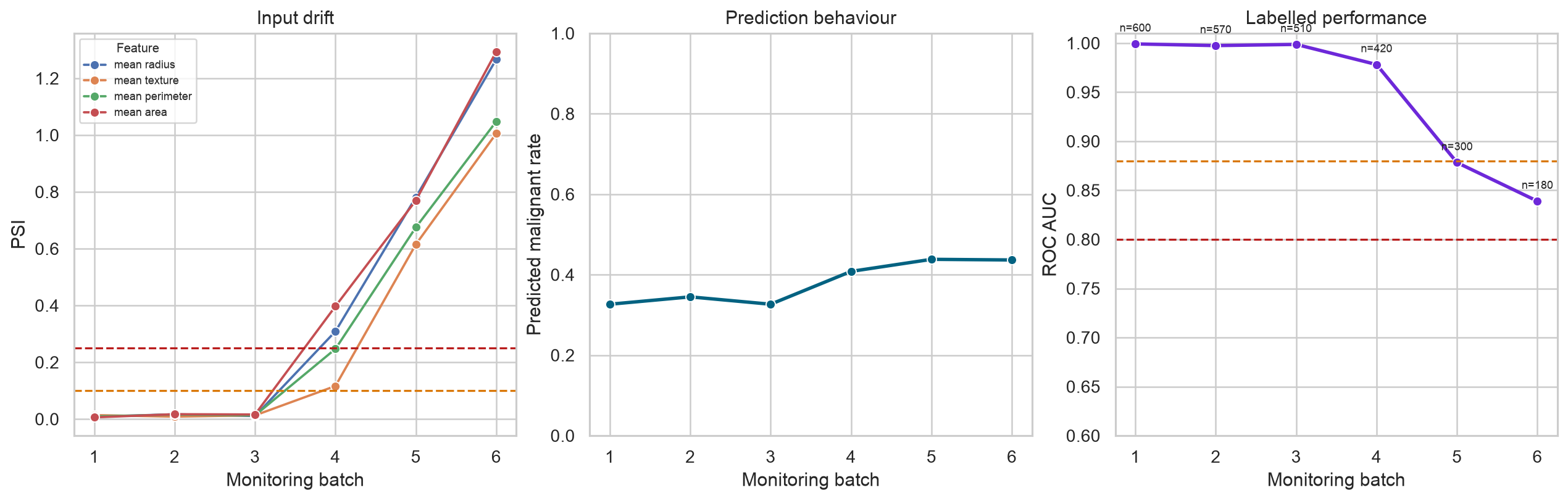
The intentional shift makes the expected sequence visible: feature drift appears immediately, prediction behaviour changes, and measured performance changes only for observations whose outcomes are available. In a real system, these signals would usually arrive through separate data paths and at different times.

From metrics to status

The demonstration assigns each metric one of three states:

• ok: within the expected operating region;
• warning: investigate and increase attention;
• critical: initiate the response defined in the runbook.

Thresholds in the script are deliberately illustrative. Production thresholds should be derived from historical variation, sample size, model risk, operational capacity, and the cost of missed detection. A reasonable policy also includes persistence—for example, warning only after two consecutive abnormal batches—so a small transient fluctuation does not page a responder.

Avoid combining all signals into one score. A single number obscures whether the response should focus on a data contract, a population change, a model problem, or incomplete labels.

Segment before concluding

Aggregate metrics can conceal local failures. Compare data quality, prediction behaviour, and performance across segments that are operationally meaningful and legally appropriate, such as collection site, device type, workflow route, or validated demographic groups.

Segment monitoring introduces two risks:

1. Small groups produce noisy estimates and may require longer windows or uncertainty intervals.
2. Monitoring sensitive attributes creates privacy and governance responsibilities.

Define access controls, retention, minimum group sizes, and escalation rules before collecting subgroup fields merely because they might be useful later.

A practical monitoring record

A batch-level record should be append-only and reproducible. A compact schema is:

Field	Purpose
window_start, window_end	observation period
model_version, data_version	traceability
segment	scoped analysis, with all for aggregate
metric_name, metric_value	machine-readable result
sample_size, labelled_count	denominator and label availability
reference_id	exact comparison baseline
status, threshold_policy	evaluated state and policy version
computed_at	pipeline audit timestamp

Keep raw monitoring data separate from aggregates. Dashboards should query validated aggregates where possible, while restricted raw records remain available for authorized investigation.

Alerting and response

A useful alert states what changed, over what window, relative to which baseline, and what the responder should do next. The runbook can use this sequence:

1. Confirm that the monitoring pipeline completed and the denominator is adequate.
2. Check schema, missingness, volume, and source-system changes.
3. Locate affected features, segments, sites, or model versions.
4. Compare prediction changes with available outcomes.
5. Assess user and decision impact.
6. Choose a response: continue observing, repair the data path, adjust the workflow, roll back, restrict use, or begin a reviewed model update.
7. Record the evidence, decision, owner, and follow-up time.

Drift should not trigger automatic retraining by itself. Retraining on corrupted, selectively labelled, or poorly understood data can preserve the failure in a new model version. Chapter 09 develops the governed feedback and retraining workflow that follows monitoring evidence.

Production implementation pattern

A mature implementation separates collection, calculation, storage, visualization, and response:

flowchart TD
    A["Inference events"] --> B["Validated monitoring store"]
    C["Delayed outcomes"] --> B
    D["Versioned reference"] --> E["Scheduled metric job"]
    B --> E
    E --> F["Metrics and dashboard"]
    F --> G["Alert and runbook"]

The metric job must be idempotent: rerunning the same window with the same reference and policy should produce the same result. Backfills should be distinguishable from live calculations, and revised outcomes should create a new computation version rather than silently changing history.

Chapter checkpoint

Before treating data and model monitoring as operationally ready, confirm that:

• each deployed model has a versioned reference dataset;
• data-quality checks precede drift calculations;
• input, prediction, and performance signals remain distinct;
• every metric includes its window and denominator;
• delayed labels are joined through stable identifiers;
• important segments are monitored with privacy safeguards;
• thresholds and persistence rules are versioned policy;
• alerts link to an owner and response runbook;
• drift initiates investigation rather than unreviewed retraining;
• monitoring outputs are reproducible and auditable.

Summary

Data and model monitoring extends observability from software behaviour to statistical behaviour. Data-quality and drift signals can reveal changes early, prediction monitoring shows how those changes propagate through the model, and delayed outcomes establish whether decision quality has actually changed. The central discipline is to preserve the distinction between evidence and conclusion: monitoring identifies where investigation is needed, while a governed response determines what should change.